N-MNIST Classification

N-MNIST is the neuromorphic version of MNIST digit recognition. The MNIST digits are converted into event based data using a DVS sensor moving in a repatable tri-saccadic motion each about 100 ms long.

The task is to classify each event sequence to it’s corresponding digit.

NMNIST dataset is freely available here (© CC-4.0).

Orchard, G.; Cohen, G.; Jayawant, A.; and Thakor, N. “Converting Static Image Datasets to Spiking Neuromorphic Datasets Using Saccades”, Frontiers in Neuroscience, vol.9, no.437, Oct. 2015

import os, sys
import glob
import zipfile
import h5py
import numpy as np
import matplotlib.pyplot as plt
import torch
from torch.utils.data import Dataset, DataLoader

# import slayer from lava-dl
import lava.lib.dl.slayer as slayer

import IPython.display as display
from matplotlib import animation

Create Dataset

The dataset class follows standard torch dataset definition. They are defined in nmnist.py. We will just import the dataset and augmentation routine here.

from nmnist import augment, NMNISTDataset

Create Network

A slayer network definition follows standard PyTorch way using torch.nn.Module.

The network can be described with a combination of individual synapse, dendrite, neuron and axon components. For rapid and easy development, slayer provides block interface - slayer.block - which bundles all these individual components into a single unit. These blocks can be cascaded to build a network easily. The block interface provides additional utilities for normalization (weight and neuron), dropout, gradient monitoring and network export.

In the example below, slayer.block.cuba is illustrated.

class Network(torch.nn.Module):
    def __init__(self):
        super(Network, self).__init__()

        neuron_params = {
                'threshold'     : 1.25,
                'current_decay' : 0.25,
                'voltage_decay' : 0.03,
                'tau_grad'      : 0.03,
                'scale_grad'    : 3,
                'requires_grad' : True,
            }
        neuron_params_drop = {**neuron_params, 'dropout' : slayer.neuron.Dropout(p=0.05),}

        self.blocks = torch.nn.ModuleList([
                slayer.block.cuba.Dense(neuron_params_drop, 34*34*2, 512, weight_norm=True, delay=True),
                slayer.block.cuba.Dense(neuron_params_drop, 512, 512, weight_norm=True, delay=True),
                slayer.block.cuba.Dense(neuron_params, 512, 10, weight_norm=True),
            ])

    def forward(self, spike):
        for block in self.blocks:
            spike = block(spike)
        return spike

    def grad_flow(self, path):
        # helps monitor the gradient flow
        grad = [b.synapse.grad_norm for b in self.blocks if hasattr(b, 'synapse')]

        plt.figure()
        plt.semilogy(grad)
        plt.savefig(path + 'gradFlow.png')
        plt.close()

        return grad

    def export_hdf5(self, filename):
        # network export to hdf5 format
        h = h5py.File(filename, 'w')
        layer = h.create_group('layer')
        for i, b in enumerate(self.blocks):
            b.export_hdf5(layer.create_group(f'{i}'))

Instantiate Network, Optimizer, DataSet and DataLoader

Running the network in GPU is as simple as selecting torch.device('cuda').

trained_folder = 'Trained'
os.makedirs(trained_folder, exist_ok=True)

# device = torch.device('cpu')
device = torch.device('cuda')

net = Network().to(device)

optimizer = torch.optim.Adam(net.parameters(), lr=0.001)

training_set = NMNISTDataset(train=True, transform=augment)
testing_set  = NMNISTDataset(train=False)

train_loader = DataLoader(dataset=training_set, batch_size=32, shuffle=True)
test_loader  = DataLoader(dataset=testing_set , batch_size=32, shuffle=True)

NMNIST dataset is freely available here: https://www.garrickorchard.com/datasets/n-mnist

(c) Creative Commons:
    Orchard, G.; Cohen, G.; Jayawant, A.; and Thakor, N.
    "Converting Static Image Datasets to Spiking Neuromorphic Datasets Using Saccades",
    Frontiers in Neuroscience, vol.9, no.437, Oct. 2015

Visualize the input data

A slayer.io.Event can be visualized by invoking it’s Event.show() routine. Event.anim() instead returns the event visualization animation which can be embedded in notebook or exported as video/gif. Here, we will export gif animation and visualize it.

for i in range(5):
    spike_tensor, label = testing_set[np.random.randint(len(testing_set))]
    spike_tensor = spike_tensor.reshape(2, 34, 34, -1)
    event = slayer.io.tensor_to_event(spike_tensor.cpu().data.numpy())
    anim = event.anim(plt.figure(figsize=(5, 5)), frame_rate=240)
    anim.save(f'gifs/input{i}.gif', animation.PillowWriter(fps=24), dpi=300)

gif_td = lambda gif: f'<td> <img src="{gif}" alt="Drawing" style="height: 250px;"/> </td>'
header = '<table><tr>'
images = ' '.join([gif_td(f'gifs/input{i}.gif') for i in range(5)])
footer = '</tr></table>'
display.HTML(header + images + footer)

Error module

Slayer provides prebuilt loss modules: slayer.loss.{SpikeTime, SpikeRate, SpikeMax}. * SpikeTime: precise spike time based loss when target spike train is known. * SpikeRate: spike rate based loss when desired rate of the output neuron is known. * SpikeMax: negative log likelihood losses for classification without any rate tuning.

Since the target spike train is not known for this problem, we use SpikeRate loss and target high spiking rate for true class and low spiking rate for false class.

target rate: \hat{\boldsymbol r} = r_\text{true}\,{\bf 1}[\text{label}] + r_\text{false}\,(1-{\bf 1}[\text{label}]) where {\bf 1}[\text{label}] is one-hot encoding of label. The loss is:

L = \frac{1}{2} \left(\frac{1}{T}\int_T {\boldsymbol s}(t)\,\text dt - \hat{\boldsymbol r}\right)^\top {\bf 1}

error = slayer.loss.SpikeRate(true_rate=0.2, false_rate=0.03, reduction='sum').to(device)

Stats and Assistants

Slayer provides slayer.utils.LearningStats as a simple learning statistics logger for training, validation and testing.

In addtion, slayer.utils.Assistant module wraps common training validation and testing routine which help simplify the training routine.

stats = slayer.utils.LearningStats()
assistant = slayer.utils.Assistant(net, error, optimizer, stats, classifier=slayer.classifier.Rate.predict)

Training Loop

Training loop mainly consists of looping over epochs and calling assistant.train and assistant.test utilities over training and testing dataset. The assistant utility takes care of statndard backpropagation procedure internally.

• stats can be used in print statement to get formatted stats printout.

• stats.testing.best_accuracy can be used to find out if the current iteration has the best testing accuracy. Here, we use it to save the best model.

• stats.update() updates the stats collected for the epoch.

• stats.save saves the stats in files.

epochs = 100

for epoch in range(epochs):
    for i, (input, label) in enumerate(train_loader): # training loop
        output = assistant.train(input, label)
    print(f'\r[Epoch {epoch:2d}/{epochs}] {stats}', end='')

    for i, (input, label) in enumerate(test_loader): # training loop
        output = assistant.test(input, label)
    print(f'\r[Epoch {epoch:2d}/{epochs}] {stats}', end='')

    if epoch%20 == 19: # cleanup display
        print('\r', ' '*len(f'\r[Epoch {epoch:2d}/{epochs}] {stats}'))
        stats_str = str(stats).replace("| ", "\n")
        print(f'[Epoch {epoch:2d}/{epochs}]\n{stats_str}')

    if stats.testing.best_accuracy:
        torch.save(net.state_dict(), trained_folder + '/network.pt')
    stats.update()
    stats.save(trained_folder + '/')
    net.grad_flow(trained_folder + '/')

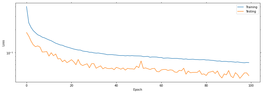
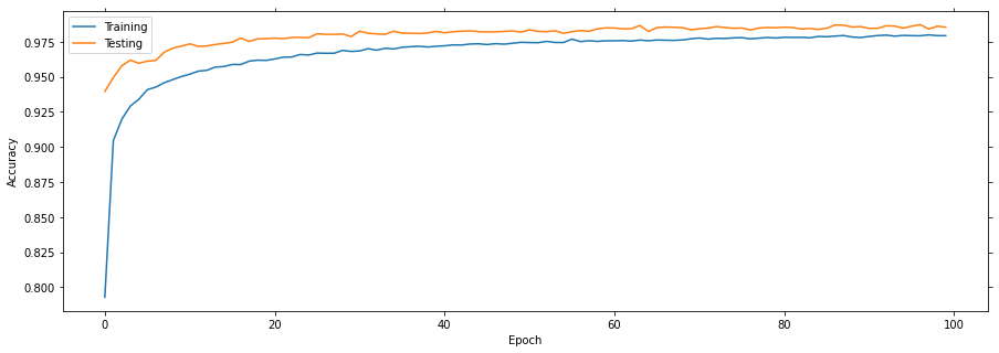
[Epoch 19/100]
Train loss =     0.11669 (min =     0.11887)    accuracy = 0.96173 (max = 0.96188)
Test  loss =     0.07722 (min =     0.07424)    accuracy = 0.97720 (max = 0.97770)

[Epoch 39/100]
Train loss =     0.09383 (min =     0.09434)    accuracy = 0.97182 (max = 0.97180)
Test  loss =     0.06004 (min =     0.06169)    accuracy = 0.98240 (max = 0.98250)

[Epoch 59/100]
Train loss =     0.08660 (min =     0.08739)    accuracy = 0.97570 (max = 0.97692)
Test  loss =     0.05640 (min =     0.05682)    accuracy = 0.98490 (max = 0.98420)

[Epoch 79/100]
Train loss =     0.08141 (min =     0.08102)    accuracy = 0.97768 (max = 0.97808)
Test  loss =     0.05284 (min =     0.05230)    accuracy = 0.98500 (max = 0.98660)

[Epoch 99/100]
Train loss =     0.07434 (min =     0.07396)    accuracy = 0.97933 (max = 0.97993)
Test  loss =     0.05019 (min =     0.04633)    accuracy = 0.98540 (max = 0.98720)

Plot the learning curves

Plotting the learning curves is as easy as calling stats.plot().

stats.plot(figsize=(15, 5))

Export the best model

Load the best model during training and export it as hdf5 network. It is supported by lava.lib.dl.netx to automatically load the network as a lava process.

net.load_state_dict(torch.load(trained_folder + '/network.pt'))
net.export_hdf5(trained_folder + '/network.net')

Visualize the network output

Here, we will use slayer.io.tensor_to_event method to convert the torch output spike tensor into slayer.io.Event object and visualize a few input and output event pairs.

output = net(input.to(device))
for i in range(5):
    inp_event = slayer.io.tensor_to_event(input[i].cpu().data.numpy().reshape(2, 34, 34, -1))
    out_event = slayer.io.tensor_to_event(output[i].cpu().data.numpy().reshape(1, 10, -1))
    inp_anim = inp_event.anim(plt.figure(figsize=(5, 5)), frame_rate=240)
    out_anim = out_event.anim(plt.figure(figsize=(10, 5)), frame_rate=240)
    inp_anim.save(f'gifs/inp{i}.gif', animation.PillowWriter(fps=24), dpi=300)
    out_anim.save(f'gifs/out{i}.gif', animation.PillowWriter(fps=24), dpi=300)

html = '<table>'
html += '<tr><td align="center"><b>Input</b></td><td><b>Output</b></td></tr>'
for i in range(5):
    html += '<tr>'
    html += gif_td(f'gifs/inp{i}.gif')
    html += gif_td(f'gifs/out{i}.gif')
    html += '</tr>'
html += '</tr></table>'
display.HTML(html)

Input	Output