Copyright (C) 2022 Intel Corporation SPDX-License-Identifier: BSD-3-Clause See: https://spdx.org/licenses/
Walk through Lava
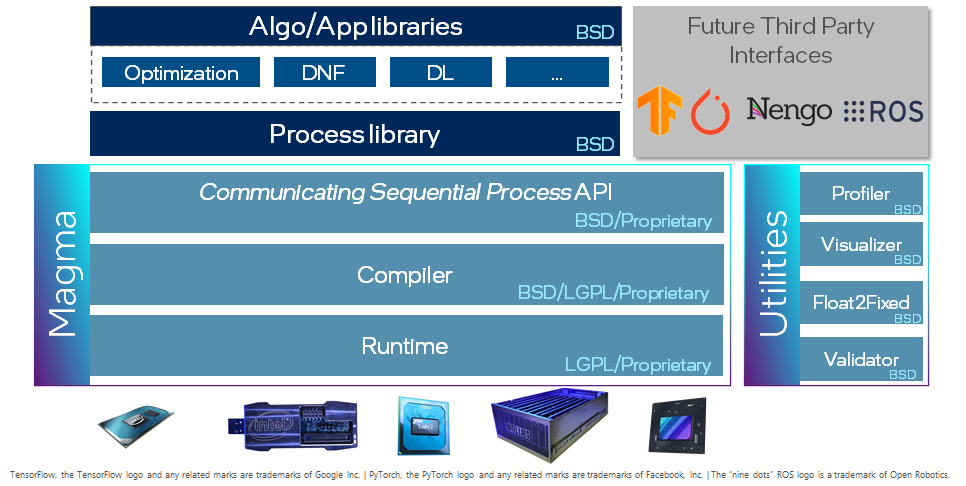
Lava is an open-source software library dedicated to the development of algorithms for neuromorphic computation. To that end, Lava provides an easy-to-use Python interface for creating the bits and pieces required for such a neuromorphic algorithm. For easy development, Lava allows to run and test all neuromorphic algorithms on standard von-Neumann hardware like CPU, before they can be deployed on neuromorphic processors such as the Intel Loihi 1/2 processor to leverage their speed and power advantages. Furthermore, Lava is designed to be extensible to custom implementations of neuromorphic behavior and to support new hardware backends.
Lava can fundamentally be used at two different levels: Either by using existing resources which can be used to create complex algorithms while requiring almost no deep neuromorphic knowledge. Or, for custom behavior, Lava can be easily extended with new behavior defined in Python and C.
This tutorial gives an high-level overview over the key components of Lava. For illustration, we will use a simple working example: a feed-forward multi-layer LIF network executed locally on CPU. In the first section of the tutorial, we use the internal resources of Lava to construct such a network and in the second section, we demonstrate how to extend Lava with a custom process using the example of an input generator.
In addition to the core Lava library described in the present tutorial, the following tutorials guide you to use high level functionalities: - lava-dl for deep learning applications - lava-optimization for constraint optimization - lava-dnf for Dynamic Neural Fields
1. Usage of the Process Library
In this section, we will use a simple 2-layered feed-forward network of LIF neurons executed on CPU as canonical example.
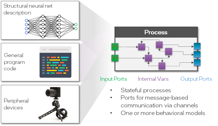
The fundamental building block in the Lava architecture is the Process. A Process describes a functional group, such as a population of LIF neurons, which runs asynchronously and parallel and communicates via Channels. A Process can take different forms and does not necessarily be a population of neurons, for example it could be a complete network, program code or the interface to a sensor (see figure below).
For convenience, Lava provides a growing Process Library in which many commonly used Processes are publicly available. In the first section of this tutorial, we will use the Processes of the Process Library to create and execute a multi-layer LIF network. Take a look at the documentation to find out what other Processes are implemented in the Process Library.
Let’s start by importing the classes LIF and Dense and take a brief look at the docstring.
[1]:
from lava.proc.lif.process import LIF
from lava.proc.dense.process import Dense

LIF?
Init signature: LIF(*args, **kwargs)
Docstring:
Leaky-Integrate-and-Fire (LIF) neural Process.

LIF dynamics abstracts to:
u[t] = u[t-1] * (1-du) + a_in         # neuron current
v[t] = v[t-1] * (1-dv) + u[t] + bias  # neuron voltage
s_out = v[t] > vth                    # spike if threshold is exceeded
v[t] = 0                              # reset at spike

Parameters
----------
shape : tuple(int)
    Number and topology of LIF neurons.
u : float, list, numpy.ndarray, optional
    Initial value of the neurons' current.
v : float, list, numpy.ndarray, optional
    Initial value of the neurons' voltage (membrane potential).
du : float, optional
    Inverse of decay time-constant for current decay. Currently, only a
    single decay can be set for the entire population of neurons.
dv : float, optional
    Inverse of decay time-constant for voltage decay. Currently, only a
    single decay can be set for the entire population of neurons.
bias_mant : float, list, numpy.ndarray, optional
    Mantissa part of neuron bias.
bias_exp : float, list, numpy.ndarray, optional
    Exponent part of neuron bias, if needed. Mostly for fixed point
    implementations. Ignored for floating point implementations.
vth : float, optional
    Neuron threshold voltage, exceeding which, the neuron will spike.
    Currently, only a single threshold can be set for the entire
    population of neurons.

Example
-------
>>> lif = LIF(shape=(200, 15), du=10, dv=5)
This will create 200x15 LIF neurons that all have the same current decay
of 10 and voltage decay of 5.
Init docstring: Initializes a new Process.
File:           ~/Documents/lava/src/lava/proc/lif/process.py
Type:           ProcessPostInitCaller
Subclasses:     LIFReset
The docstring gives insights about the parameters and internal dynamics of the LIF neuron. Dense is used to connect to a neuron population in an all-to-all fashion, often implemented as a matrix-vector product.
In the next box, we will create the Processes we need to implement a multi-layer LIF (LIF-Dense-LIF) network.
[2]:
import numpy as np

# Create processes
lif1 = LIF(shape=(3, ),                         # Number and topological layout of units in the process
           vth=10.,                             # Membrane threshold
           dv=0.1,                              # Inverse membrane time-constant
           du=0.1,                              # Inverse synaptic time-constant
           bias_mant=(1.1, 1.2, 1.3),           # Bias added to the membrane voltage in every timestep
           name="lif1")

dense = Dense(weights=np.random.rand(2, 3),     # Initial value of the weights, chosen randomly
              name='dense')

lif2 = LIF(shape=(2, ),                         # Number and topological layout of units in the process
           vth=10.,                             # Membrane threshold
           dv=0.1,                              # Inverse membrane time-constant
           du=0.1,                              # Inverse synaptic time-constant
           bias_mant=0.,                        # Bias added to the membrane voltage in every timestep
           name='lif2')
As you can see, we can either specify parameters with scalars, then all units share the same initial value for this parameter, or with a tuple (or list, or numpy array) to set the parameter individually per unit.
Processes
Let’s investigate the objects we just created. As mentioned before, both, LIF and Dense are examples of Processes, the main building block in Lava.
A Process holds three key components (see figure below):
Input ports
Variables
Output ports
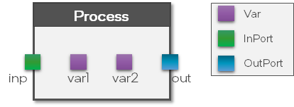
The Vars are used to store internal states of the Process while the Ports are used to define the connectivity between the Processes. Note that a Process only defines the Vars and Ports but not the behavior. This is done separately in a ProcessModel. To separate the interface from the behavioral implementation has the advantage that we can define the behavior of a Process for multiple hardware backends using multiple ProcessModels without changing the
interface. We will get into more detail about ProcessModels in the second part of this tutorial.
Ports and connections
Let’s take a look at the Ports of the LIF and Dense processes we just created. The output Port of the LIF neuron is called s_out, which stands for ‘spiking’ output. The input Port is called a_in which stands for ‘activation’ input.
For example, we can see the size of the Port which is in particular important because Ports can only connect if their shape matches.
[3]:
for proc in [lif1, lif2, dense]:
    for port in proc.in_ports:
        print(f'Proc: {proc.name:<5}  Name: {port.name:<5}  Size: {port.size}')
    for port in proc.out_ports:
        print(f'Proc: {proc.name:<5}  Name: {port.name:<5}  Size: {port.size}')
Proc: lif1   Name: a_in   Size: 3
Proc: lif1   Name: s_out  Size: 3
Proc: lif2   Name: a_in   Size: 2
Proc: lif2   Name: s_out  Size: 2
Proc: dense  Name: s_in   Size: 3
Proc: dense  Name: a_out  Size: 2
Now that we know about the input and output Ports of the LIF and Dense Processes, we can connect the network to complete the LIF-Dense-LIF structure.
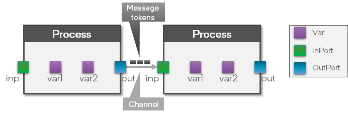
As can be seen in the figure above, by connecting two processes, a Channel between them is created which means that messages between those two Processes can be exchanged.
[4]:
lif1.s_out.connect(dense.s_in)
dense.a_out.connect(lif2.a_in)
Variables
Similar to the Ports, we can investigate the Vars of a Process.
Vars are also accessible as member variables. We can print details of a specific Var to see the shape, initial value and current value. The shareable attribute controls whether a Var can be manipulated via remote memory access. Learn more about about this topic in the remote memory access tutorial.
[5]:
for var in lif1.vars:
    print(f'Var: {var.name:<9}  Shape: {var.shape}  Init: {var.init}')
Var: bias_exp   Shape: (3,)  Init: 0
Var: bias_mant  Shape: (3,)  Init: (1.1, 1.2, 1.3)
Var: du         Shape: (1,)  Init: 0.1
Var: dv         Shape: (1,)  Init: 0.1
Var: u          Shape: (3,)  Init: 0
Var: v          Shape: (3,)  Init: 0
Var: vth        Shape: (1,)  Init: 10.0
We can take a look at the random weights of Dense by calling the get function.
Note: There is also a set function available to change the value of a Var after the network was executed.
[6]:
dense.weights.get()
[6]:
array([[0.39348157, 0.11634913, 0.17421253],
       [0.51148951, 0.9046173 , 0.04863679]])
Record internal Vars over time
In order to record the evolution of the internal Vars over time, we need a Monitor. For this example, we want to record the membrane potential of both LIF Processes, hence we need two Monitors.
We can define the Var that a Monitor should record, as well as the recording duration, using the probe function.
[7]:
from lava.proc.monitor.process import Monitor

monitor_lif1 = Monitor()
monitor_lif2 = Monitor()

num_steps = 100

monitor_lif1.probe(lif1.v, num_steps)
monitor_lif2.probe(lif2.v, num_steps)
Execution
Now, that we finished to set up the network and recording Processes, we can execute the network by simply calling the run function of one of the Processes.
The run function requires two parameters, a RunCondition and a RunConfig. The RunCondition defines how the network runs (i.e. for how long) while the RunConfig defines on which hardware backend the Processes should be mapped and executed.
Run Conditions
Let’s investigate the different possibilities for RunConditions. One option is RunContinuous which executes the network continuously and non-blocking until pause or stop is called.
[8]:
from lava.magma.core.run_conditions import RunContinuous

run_condition = RunContinuous()
The second option is RunSteps, which allows you to define an exact amount of time steps the network should run.
[9]:
from lava.magma.core.run_conditions import RunSteps

run_condition = RunSteps(num_steps=num_steps)
For this example. we will use RunSteps and let the network run exactly num_steps time steps.
RunConfigs
Next, we need to provide a RunConfig. As mentioned above, The RunConfig defines on which hardware backend the network is executed.
For example, we could run the network on the Loihi1 processor using the Loihi1HwCfg, on Loihi2 using the Loihi2HwCfg, or on CPU using the Loihi1SimCfg. The compiler and runtime then automatically select the correct ProcessModels such that the RunConfig can be fulfilled.
For this section of the tutorial, we will run our network on CPU, later we will show how to run the same network on the Loihi2 processor.
[10]:
from lava.magma.core.run_configs import Loihi1SimCfg

run_cfg = Loihi1SimCfg(select_tag="floating_pt")
Execute
Finally, we can simply call the run function of the second LIF process and provide the RunConfig and RunCondition.
[11]:
lif2.run(condition=run_condition, run_cfg=run_cfg)
Retrieve recorded data
After the simulation has stopped, we can call get_data on the two monitors to retrieve the recorded membrane potentials.
[12]:
data_lif1 = monitor_lif1.get_data()
data_lif2 = monitor_lif2.get_data()
Alternatively, we can also use the provided plot functionality of the Monitor, to plot the recorded data. As we can see, the bias of the first LIF population drives the membrane potential to the threshold which generates output spikes. Those output spikes are passed through the Dense layer as input to the second LIF population.
[13]:
import matplotlib
%matplotlib inline
from matplotlib import pyplot as plt

# Create a subplot for each monitor
fig = plt.figure(figsize=(16, 5))
ax0 = fig.add_subplot(121)
ax1 = fig.add_subplot(122)

# Plot the recorded data
monitor_lif1.plot(ax0, lif1.v)
monitor_lif2.plot(ax1, lif2.v)

As a last step we must stop the runtime by calling the stop function. Stop will terminate the Runtime and all states will be lost.
[14]:
lif2.stop()
Summary
There are many tools available in the Process Library to construct basic networks
The fundamental building block in Lava is the
ProcessEach
Processconsists ofVarsandPortsA
Processdefines a common interface across hardware backends, but not the behaviorThe
ProcessModeldefines the behavior of aProcessfor a specific hardware backendVarsstore internal states,Portsare used to implement communication channels between processesThe
RunConfigdefines on which hardware backend the network runs
Learn more about
2. Create a custom Process
In the previous section of this tutorial, we used Processes which were available in the Process Library. In many cases, this might be sufficient and the Process Library is constantly growing. Nevertheless, the Process Library can not cover all use-cases. Hence, Lava makes it very easy to create new Processes. In the following section, we want to show how to implement a custom Process and the corresponding behavior using a ProcessModel.
The example of the previous section implemented a bias driven LIF-Dense-LIF network. One crucial aspect which is missing this example, is the input/output interaction with sensors and actuators. Commonly used sensors would be Dynamic Vision Sensors or artificial cochleas, but for demonstration purposes we will implement a simple SpikeGenerator. The purpose of the SpikeGenerator is to output random spikes to drive the LIF-Dense-LIF network.
Let’s start by importing the necessary classes from Lava.
[15]:
from lava.magma.core.process.process import AbstractProcess
from lava.magma.core.process.variable import Var
from lava.magma.core.process.ports.ports import OutPort
All Processes in Lava inherit from a common base class called AbstractProcess. Additionally, we need Var for storing the spike probability and OutPort to define the output connections for our SpikeGenerator.
[16]:
class SpikeGenerator(AbstractProcess):
    """Spike generator process provides spikes to subsequent Processes.

    Parameters
    ----------
    shape: tuple
        defines the dimensionality of the generated spikes per timestep
    spike_prob: int
        spike probability in percent
    """
    def __init__(self, shape: tuple, spike_prob: int) -> None:
        super().__init__()
        self.spike_prob = Var(shape=(1, ), init=spike_prob)
        self.s_out = OutPort(shape=shape)
The constructor of Var requires the shape of the data to be stored and some initial value. We use this functionality to store the spike data. Similarly, we define an OutPort for our SpikeGenerator.
Create a new ProcessModel
As mentioned earlier, the Process only defines the interface but not the behavior of the SpikeGenerator. We will do that in a separate ProcessModel which has the advantage that we can define the behavior of a Process on different hardware backends without changing the interface (see figure below). More details about the different kinds of ProcessModels can be found in the dedicated in-depth tutorials
(here and here). Lava automatically selects the correct ProcessModel for each Process given the RunConfig.
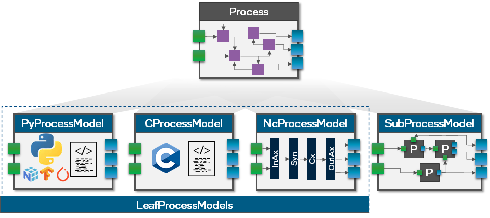
So, let’s go ahead and define the behavior of the SpikeGenerator on a CPU in Python. Later in this tutorial we will show how to implement the same behavior on an embedded CPU in C and how to implement the behavior of a LIF process on a Loihi2 neuro-core.
We first import all necessary classes from Lava.
[17]:
from lava.magma.core.model.py.model import PyLoihiProcessModel
from lava.magma.core.resources import CPU
from lava.magma.core.decorator import implements, requires
from lava.magma.core.sync.protocols.loihi_protocol import LoihiProtocol
from lava.magma.core.model.py.type import LavaPyType
from lava.magma.core.model.py.ports import PyOutPort
All ProcessModels defined to run on CPU are written in Python and inherit from the common class called PyLoihiProcessModel. Further, we use the decorators requires and implements to define which computational resources (i.e. CPU, GPU, Loihi1NeuroCore, Loihi2NeuroCore) are required to execute this ProcessModel and which Process it implements. Finally, we need to specify the types of Vars and Ports in our SpikeGenerator using LavaPyType and PyOutPort.
Note: It is important to mention that the ProcessModel needs to implement the exact same Vars and Ports of the parent process using the same class attribute names.
Additionally, we define that our PySpikeGeneratorModel follows the LoihiProtocol. The LoihiProtocol defines that the execution of a model follows a specific sequence of phases. For example, there is the spiking phase (run_spk) in which input spikes are received, internal Vars are updated and output spikes are sent. There are other phases such as the learning phase (run_lrn) in which online learning takes place, or the post management phase (run_post_mgmt) in
which memory content is updated. As the SpikeGenerator basically just sends out spikes, the correct place to implement its behavior is the run_spk phase.
To implement the behavior, we need to have access to the global simulation time. We can easily access the simulation time with self.time_step and use that to index the spike_data and send out the corresponding spikes through the OutPort.
[18]:
@implements(proc=SpikeGenerator, protocol=LoihiProtocol)
@requires(CPU)
class PySpikeGeneratorModel(PyLoihiProcessModel):
    """Spike Generator process model."""
    spike_prob: int = LavaPyType(int, int)
    s_out: PyOutPort = LavaPyType(PyOutPort.VEC_DENSE, float)

    def run_spk(self) -> None:
        # Generate random spike data
        spike_data = np.random.choice([0, 1], p=[1 - self.spike_prob/100, self.spike_prob/100], size=self.s_out.shape[0])

        # Send spikes
        self.s_out.send(spike_data)
Note: For the SpikeGenerator we only needed an OutPort which provides the send function to send data. For the InPort the corresponding function to receive data is called recv.
Next, we want to redefine our network as in the example before with the exception that we turn off all biases.
[19]:
# Create processes
lif1 = LIF(shape=(3, ),                         # Number of units in this process
           vth=10.,                             # Membrane threshold
           dv=0.1,                              # Inverse membrane time-constant
           du=0.1,                              # Inverse synaptic time-constant
           bias_mant=0.,                        # Bias added to the membrane voltage in every timestep
           name="lif1")

dense = Dense(weights=np.random.rand(2, 3),     # Initial value of the weights, chosen randomly
              name='dense')

lif2 = LIF(shape=(2, ),                         # Number of units in this process
           vth=10.,                             # Membrane threshold
           dv=0.1,                              # Inverse membrane time-constant
           du=0.1,                              # Inverse synaptic time-constant
           bias_mant=0.,                        # Bias added to the membrane voltage in every timestep
           name='lif2')

# Connect the OutPort of lif1 to the InPort of dense
lif1.s_out.connect(dense.s_in)

# Connect the OutPort of dense to the InPort of lif2
dense.a_out.connect(lif2.a_in)

# Create Monitors to record membrane potentials
monitor_lif1 = Monitor()
monitor_lif2 = Monitor()

# Probe membrane potentials from the two LIF populations
monitor_lif1.probe(lif1.v, num_steps)
monitor_lif2.probe(lif2.v, num_steps)
Use the custom SpikeGenerator
We instantiate the SpikeGenerator as usual with the shape of the fist LIF population.
To define the connectivity between the SpikeGenerator and the first LIF population, we us another Dense Layer. Now, we can connect its OutPort to the InPort of the Dense layer and the OutPort of the Dense layer to the InPort of the first LIF population.
[20]:
# Instantiate SpikeGenerator
spike_gen = SpikeGenerator(shape=(lif1.a_in.shape[0], ), spike_prob=7)

# Instantiate Dense
dense_input = Dense(weights=np.eye(lif1.a_in.shape[0])) # one-to-one connectivity

# Connect spike_gen to dense_input
spike_gen.s_out.connect(dense_input.s_in)

# Connect dense_input to LIF1 population
dense_input.a_out.connect(lif1.a_in)
Execute and plot
Now that our network is complete, we can execute it the same way as before using the RunCondition and RunConfig we created in the previous example.
[21]:
lif2.run(condition=run_condition, run_cfg=run_cfg)
And now, we can retrieve the recorded data and plot the membrane potentials of the two LIF populations.
[22]:
# Create a subplot for each monitor
fig = plt.figure(figsize=(16, 5))
ax0 = fig.add_subplot(121)
ax1 = fig.add_subplot(122)

# Plot the recorded data
monitor_lif1.plot(ax0, lif1.v)
monitor_lif2.plot(ax1, lif2.v)

As we can see, the spikes provided by the SpikeGenerator are sucessfully sent to the first LIF population. which in turn sends its output spikes to the second LIF population.
[23]:
lif2.stop()
Summary
Define custom a
Processby inheritance fromAbstractProcessVarsare used to store internal data in theProcessPortsare used to connect to otherProcessesThe behavior of a
Processis defined in aProcessModelProcessModelsare aware of their hardware backend, they get selected automatically by the compiler/runtimePyProcessModelsrun on CPUNumber and names of
VarsandPortsof aProcessModelmust match those of theProcessit implements
Learn more about
How to learn more?
If you want to find out more about Lava, have a look at the Lava documentation or dive deeper with the in-depth tutorials.
To receive regular updates on the latest developments and releases of the Lava Software Framework please subscribe to our newsletter.