Spike to Spike Regression: Oxford

This tutorial demonstrates spike to spike regression training using ``lava.lib.dl.slayer``.

The task is to learn to transform a random Poisson spike train to produce output spike pattern that resembles The Radcliffe Camera building of Oxford University, England. The input and output both consist of 200 neurons each and the spikes span approximately 1900ms. The input and output pair are converted from SuperSpike (© GPL-3).

Input	Target

import os
import h5py
import numpy as np
import matplotlib.pyplot as plt
import torch
from torch.utils.data import Dataset, DataLoader

# import slayer from lava-dl
import lava.lib.dl.slayer as slayer

import IPython.display as display
from matplotlib import animation

Create Dataset

Create a simple PyTorch dataset class. The dataset class follows standard torch dataset definition.

It shows usage of ``slayer.io`` module. The module provides a way to

• easily represent events including graded spikes

• read/write events in different known binary and numpy formats

• transform event to tensor for processing it using slayer network and convert a spike tensor back to event

• display/animate the tensor for visualization

class OxfordDataset(Dataset):
    def __init__(self):
        super(OxfordDataset, self).__init__()
        self.input  = slayer.io.read_1d_spikes('input.bs1' )
        self.target = slayer.io.read_1d_spikes('output.bs1')
        self.target.t = self.target.t.astype(int)

    def __getitem__(self, _):
        return (
            self.input.fill_tensor(torch.zeros(1, 1, 200, 2000)).squeeze(),  # input
            self.target.fill_tensor(torch.zeros(1, 1, 200, 2000)).squeeze(), # target
        )

    def __len__(self):
        return 1 # just one sample for this problem

Create Network

A slayer network definition follows standard PyTorch way using torch.nn.Module.

The network can be described with a combination of individual synapse, dendrite, neuron and axon components. For rapid and easy development, slayer provides block interface - slayer.block - which bundles all these individual components into a single unit. These blocks can be cascaded to build a network easily. The block interface provides additional utilities for normalization (weight and neuron), dropout, gradient monitoring and network export.

In the example below, slayer.block.cuba is illustrated.

class Network(torch.nn.Module):
    def __init__(self):
        super(Network, self).__init__()

        neuron_params = {
                'threshold'     : 0.1,
                'current_decay' : 1,
                'voltage_decay' : 0.1,
                'requires_grad' : True,
            }

        self.blocks = torch.nn.ModuleList([
                slayer.block.cuba.Dense(neuron_params, 200, 256),
                slayer.block.cuba.Dense(neuron_params, 256, 200),
            ])

    def forward(self, spike):
        for block in self.blocks:
            spike = block(spike)
        return spike

    def export_hdf5(self, filename):
        # network export to hdf5 format
        h = h5py.File(filename, 'w')
        layer = h.create_group('layer')
        for i, b in enumerate(self.blocks):
            b.export_hdf5(layer.create_group(f'{i}'))

Instantiate Network, Optimizer, DataSet and DataLoader

Running the network in GPU is as simple as selecting torch.device('cuda').

trained_folder = 'Trained'
os.makedirs(trained_folder, exist_ok=True)

# device = torch.device('cpu')
device = torch.device('cuda')

net = Network().to(device)

optimizer = torch.optim.Adam(net.parameters(), lr=0.001, weight_decay=1e-5)

training_set = OxfordDataset()
train_loader = DataLoader(dataset=training_set, batch_size=1)

Visualize the input and output spike train

A slayer.io.Event can be visualized by invoking it’s Event.show() routine. Event.anim() instead returns the event visualization animation which can be embedded in notebook or exported as video/gif. Here, we will export gif animation and visualize it.

input_anim  = training_set.input.anim(plt.figure(figsize=(10, 10)))
target_anim = training_set.target.anim(plt.figure(figsize=(10, 10)))

## This produces interactive animation
# display.HTML(input_anim.to_jshtml())
# display.HTML(target_anim.to_jshtml())

## Saving and loading gif for better animation in github
input_anim.save('input.gif', animation.PillowWriter(fps=24), dpi=300)
target_anim.save('target.gif', animation.PillowWriter(fps=24), dpi=300)

gif_td = lambda gif: f'<td> <img src="{gif}" alt="Drawing" style="height: 400px;"/> </td>'
html = '<table><tr>'
html += '<td> Input </td><td> Target </td></tr><tr>'
html += gif_td(f'input.gif')
html += gif_td(f'target.gif')
html += '</tr></table>'
display.HTML(html)

Input	Target

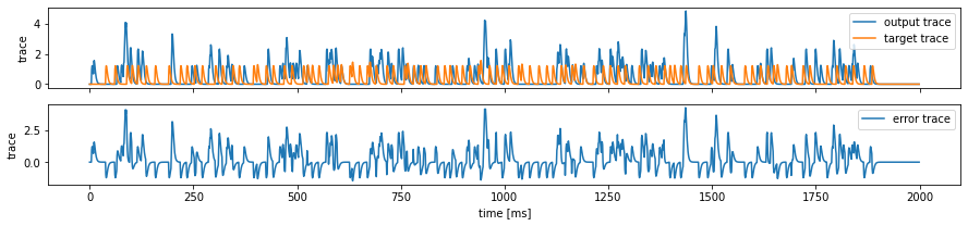
Error module

Slayer provides prebuilt loss modules: slayer.loss.{SpikeTime, SpikeRate, SpikeMax}. * SpikeTime: precise spike time based loss when target spike train is known. * SpikeRate: spike rate based loss when desired rate of the output neuron is known. * SpikeMax: negative log likelihood losses for classification without any rate tuning.

Since the target spike train \hat{\boldsymbol s}(t) is known for this problem, we use SpikeTime loss here. It uses van Rossum like spike train distance metric. The actual and target spike trains are filtered using a FIR filter and the norm of the timeseries is the loss metric.

L = \frac{1}{2T} \int_T \left(h_\text{FIR} * ({\boldsymbol s} - \hat{\boldsymbol s})\right)(t)^\top{\bf 1}\,\text dt

• time_constant: time constant of the FIR filter.

• filter_order: the order of FIR filter. Exponential decay is first order filter.

error = slayer.loss.SpikeTime(time_constant=2, filter_order=2).to(device)

# the followng portion just illustrates the SpikeTime loss calculation.
# IT IS NOT NEEDED IN PRACTICE
input, target = training_set[0]
output = net(input.unsqueeze(dim=0).to(device))[0]
# just considering first neuron for illustration
output_trace = error.filter(output[0].to(device)).flatten().cpu().data.numpy()
target_trace = error.filter(target[0].to(device)).flatten().cpu().data.numpy()
fig, ax = plt.subplots(2, 1, figsize=(15, 3), sharex=True)
ax[0].plot(output_trace, label='output trace')
ax[0].plot(target_trace, label='target trace')
ax[1].plot(output_trace - target_trace, label='error trace')
ax[0].set_ylabel('trace')
ax[1].set_ylabel('trace')
ax[1].set_xlabel('time [ms]')
for a in ax: a.legend()

Stats and Assistants

Slayer provides slayer.utils.LearningStats as a simple learning statistics logger for training, validation and testing.

In addtion, slayer.utils.Assistant module wraps common training validation and testing routine which help simplify the training routine.

stats = slayer.utils.LearningStats()
assistant = slayer.utils.Assistant(net, error, optimizer, stats)

Training Loop

Training loop mainly consists of looping over epochs and calling assistant.train utility to train.

• stats can be used in print statement to get formatted stats printout.

• stats.training.best_loss can be used to find out if the current iteration has the best loss. Here, we use it to save the best model.

• stats.update() updates the stats collected for the epoch.

• stats.save saves the stats in files.

epochs = 5000

for epoch in range(epochs):
    for i, (input, target) in enumerate(train_loader): # training loop
        output = assistant.train(input, target)
        print(f'\r[Epoch {epoch:3d}/{epochs}] {stats}', end='')

    if stats.training.best_loss:
        torch.save(net.state_dict(), trained_folder + '/network.pt')
    stats.update()
    stats.save(trained_folder + '/')

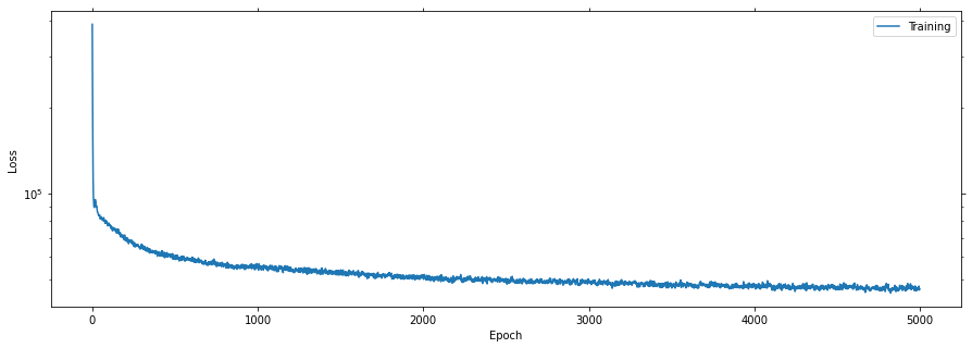
[Epoch 4999/5000] Train loss = 46478.09375 (min = 44918.71875))

Plot the learning curves

Plotting the learning curves is as easy as calling stats.plot().

stats.plot(figsize=(15, 5))

Export the best model

Load the best model during training and export it as hdf5 network. It is supported by lava.lib.dl.netx to automatically load the network as a lava process.

net.load_state_dict(torch.load(trained_folder + '/network.pt'))
net.export_hdf5(trained_folder + '/network.net')

Visualize the network output

Here, we will use slayer.io.tensor_to_event method to convert the torch output spike tensor into slayer.io.Event object and visualize the input and output event.

output = net(input.to(device))
event = slayer.io.tensor_to_event(output.cpu().data.numpy())
output_anim = event.anim(plt.figure(figsize=(10, 10)))
# display.HTML(output_anim.to_jshtml())
output_anim.save('output.gif', animation.PillowWriter(fps=24), dpi=300)

html = '<table><tr>'
html += '<td>Output</td><td>Target</td></tr><tr>'
html += gif_td(f'output.gif')
html += gif_td(f'target.gif')
html += '</tr></table>'
display.HTML(html)

Output	Target

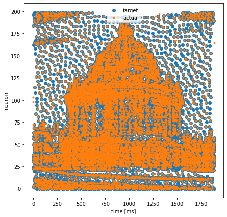
Compare Output vs Target

Event data can be accessed as slayer.io.Event.{x, y, c, t, p} for x-address, y-address, channel-address, timestamp and graded-payload. This can be used for further processing and visualization of event data.

plt.figure(figsize=(7, 7))
plt.plot(training_set.target.t, training_set.target.x, '.', markersize=12, label='target')
plt.plot(event.t, event.x, '.', label='actual')
plt.xlabel('time [ms]')
plt.ylabel('neuron')
plt.legend()

<matplotlib.legend.Legend at 0x7f78ce257430>