PilotNet Sigma-Delta Neural Network (SDNN) Training

PilotNet: Predict the car’s steering angle from the dashboard view.

PilotNet dataset is available freely here. © MIT License.

What are SDNNs?

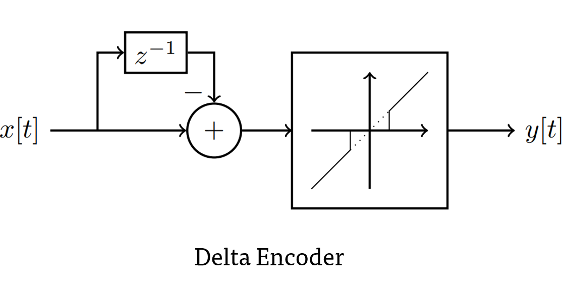
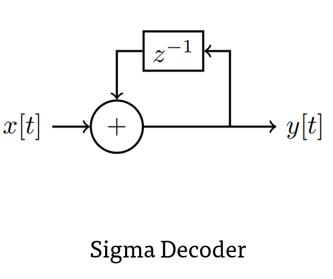
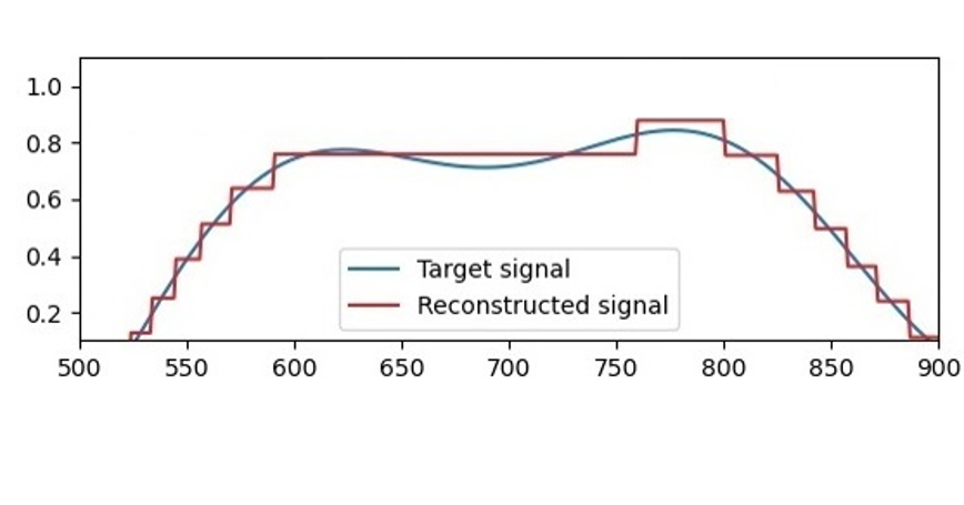
Sigma-delta neural networks consists of two main units: sigma decoder in the dendrite and delta encoder in the axon. Delta encoder uses differential encoding on the output activation of a regular ANN activation, for e.g. ReLU. In addition it only sends activation to the next layer when the encoded message magnitude is larger than its threshold. The sigma unit accumulates the sparse event messages and accumulates it to restore the original value.

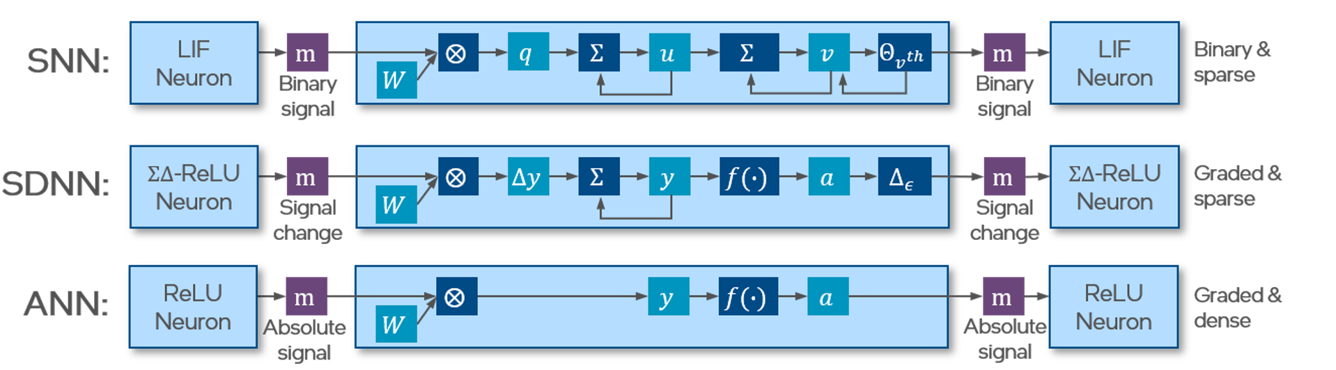
A sigma-delta neuron is simply a regular activation wrapped around by a sigma unit at it’s input and a delta unit at its output.

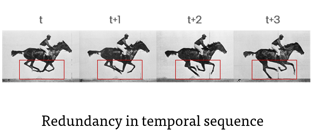
When the input to the network is a temporal sequence, the activations do not change much. Therefore, the message between the layers are reduced which in turn reduces the synaptic computation in the next layer. In addition, the graded event values can encode the change in magnitude in one time-step. Therefore there is no increase in latency at the cost of time-steps unlike the rate coded Spiking Neural Networks.

Credit Eadweard Muybridge © Public Domain

import sys, os
import numpy as np
import matplotlib.pyplot as plt
import h5py

import torch
from torch.utils.data import DataLoader
from torchvision import transforms
import torch.nn.functional as F

import lava.lib.dl.slayer as slayer

from pilotnet_dataset import PilotNetDataset
import utils

torch.manual_seed(4205)

<torch._C.Generator at 0x7fa1881d0a90>

Event sparsity loss

Sparsity loss to penalize the network for high event-rate.

def event_rate_loss(x, max_rate=0.01):
    mean_event_rate = torch.mean(torch.abs(x))
    return F.mse_loss(F.relu(mean_event_rate - max_rate), torch.zeros_like(mean_event_rate))

Network description

SLAYER 2.0 (``lava.dl.slayer``) provides a variety of learnable neuron models , synapses axons and dendrites that support quantized training. For easier use, it also provides ``block`` interface which packages the associated neurons, synapses, axons and dendrite features into a single module.

Sigma-delta blocks are available as slayer.blocks.sigma_delta.{Dense, Conv, Pool, Input, Output, Flatten, ...} which can be easily composed to create a variety of sequential network descriptions as shown below. The blocks can easily enable synaptic weight normalization, neuron normalization as well as provide useful gradient monitoring utility and hdf5 network export utility.

These blocks can be used to create a network using standard PyTorch procedure.

class Network(torch.nn.Module):
    def __init__(self):
        super(Network, self).__init__()

        sdnn_params = { # sigma-delta neuron parameters
                'threshold'     : 0.1,    # delta unit threshold
                'tau_grad'      : 0.5,    # delta unit surrogate gradient relaxation parameter
                'scale_grad'    : 1,      # delta unit surrogate gradient scale parameter
                'requires_grad' : True,   # trainable threshold
                'shared_param'  : True,   # layer wise threshold
                'activation'    : F.relu, # activation function
            }
        sdnn_cnn_params = { # conv layer has additional mean only batch norm
                **sdnn_params,                                 # copy all sdnn_params
                'norm' : slayer.neuron.norm.MeanOnlyBatchNorm, # mean only quantized batch normalizaton
            }
        sdnn_dense_params = { # dense layers have additional dropout units enabled
                **sdnn_cnn_params,                        # copy all sdnn_cnn_params
                'dropout' : slayer.neuron.Dropout(p=0.2), # neuron dropout
            }

        self.blocks = torch.nn.ModuleList([# sequential network blocks
                # delta encoding of the input
                slayer.block.sigma_delta.Input(sdnn_params),
                # convolution layers
                slayer.block.sigma_delta.Conv(sdnn_cnn_params,  3, 24, 3, padding=0, stride=2, weight_scale=2, weight_norm=True),
                slayer.block.sigma_delta.Conv(sdnn_cnn_params, 24, 36, 3, padding=0, stride=2, weight_scale=2, weight_norm=True),
                slayer.block.sigma_delta.Conv(sdnn_cnn_params, 36, 64, 3, padding=(1, 0), stride=(2, 1), weight_scale=2, weight_norm=True),
                slayer.block.sigma_delta.Conv(sdnn_cnn_params, 64, 64, 3, padding=0, stride=1, weight_scale=2, weight_norm=True),
                # flatten layer
                slayer.block.sigma_delta.Flatten(),
                # dense layers
                slayer.block.sigma_delta.Dense(sdnn_dense_params, 64*40, 100, weight_scale=2, weight_norm=True),
                slayer.block.sigma_delta.Dense(sdnn_dense_params,   100,  50, weight_scale=2, weight_norm=True),
                slayer.block.sigma_delta.Dense(sdnn_dense_params,    50,  10, weight_scale=2, weight_norm=True),
                # linear readout with sigma decoding of output
                slayer.block.sigma_delta.Output(sdnn_dense_params,   10,   1, weight_scale=2, weight_norm=True)
            ])


    def forward(self, x):
        count = []
        event_cost = 0

        for block in self.blocks:
            # forward computation is as simple as calling the blocks in a loop
            x = block(x)
            if hasattr(block, 'neuron'):
                event_cost += event_rate_loss(x)
                count.append(torch.sum(torch.abs((x[..., 1:]) > 0).to(x.dtype)).item())

        return x, event_cost, torch.FloatTensor(count).reshape((1, -1)).to(x.device)

    def grad_flow(self, path):
        # helps monitor the gradient flow
        grad = [b.synapse.grad_norm for b in self.blocks if hasattr(b, 'synapse')]

        plt.figure()
        plt.semilogy(grad)
        plt.savefig(path + 'gradFlow.png')
        plt.close()

        return grad

    def export_hdf5(self, filename):
        # network export to hdf5 format
        h = h5py.File(filename, 'w')
        layer = h.create_group('layer')
        for i, b in enumerate(self.blocks):
            b.export_hdf5(layer.create_group(f'{i}'))

Training parameters

batch  = 8  # batch size
lr     = 0.001 # leaerning rate
lam    = 0.01  # lagrangian for event rate loss
epochs = 200  # training epochs
steps  = [60, 120, 160] # learning rate reduction milestones

trained_folder = 'Trained'
logs_folder = 'Logs'

os.makedirs(trained_folder, exist_ok=True)
os.makedirs(logs_folder   , exist_ok=True)

device = torch.device('cuda')

Instantiate Network, Optimizer, Dataset and Dataloader

net = Network().to(device)

optimizer = torch.optim.RAdam(net.parameters(), lr=lr, weight_decay=1e-5)

# Datasets
training_set = PilotNetDataset(
    train=True,
    transform=transforms.Compose([
        transforms.Resize([33, 100]),
        transforms.ToTensor(),
        transforms.Normalize((0.5, 0.5, 0.5), (0.5, 0.5, 0.5)),
    ]),
)
testing_set = PilotNetDataset(
    train=False,
    transform=transforms.Compose([
        transforms.Resize([33, 100]),
        transforms.ToTensor(),
        transforms.Normalize((0.5, 0.5, 0.5), (0.5, 0.5, 0.5)),
    ]),
)

train_loader = DataLoader(dataset=training_set, batch_size=batch, shuffle=True, num_workers=8)
test_loader  = DataLoader(dataset=testing_set , batch_size=batch, shuffle=True, num_workers=8)

stats = slayer.utils.LearningStats()
assistant = slayer.utils.Assistant(
        net=net,
        error=lambda output, target: F.mse_loss(output.flatten(), target.flatten()),
        optimizer=optimizer,
        stats=stats,
        count_log=True,
        lam=lam
    )

Training loop

Training loop mainly consists of looping over epochs and calling assistant.train and assistant.test utilities over training and testing dataset. The assistant utility takes care of statndard backpropagation procedure internally.

• stats can be used in print statement to get formatted stats printout.

• stats.testing.best_loss can be used to find out if the current iteration has the best testing loss. Here, we use it to save the best model.

• stats.update() updates the stats collected for the epoch.

• stats.save saves the stats in files.

for epoch in range(epochs):
    if epoch in steps:
        for param_group in optimizer.param_groups:
            print('\nLearning rate reduction from', param_group['lr'])
            param_group['lr'] /= 10/3

    for i, (input, ground_truth) in enumerate(train_loader): # training loop
        assistant.train(input, ground_truth)
        print(f'\r[Epoch {epoch:3d}/{epochs}] {stats}', end='')

    for i, (input, ground_truth) in enumerate(test_loader): # testing loop
        assistant.test(input, ground_truth)
        print(f'\r[Epoch {epoch:3d}/{epochs}] {stats}', end='')

    if epoch%50==49: print()
    if stats.testing.best_loss:
        torch.save(net.state_dict(), trained_folder + '/network.pt')
    stats.update()
    stats.save(trained_folder + '/')

    # gradient flow monitoring
    net.grad_flow(trained_folder + '/')

    # checkpoint saves
    if epoch%10 == 0:
        torch.save({'net': net.state_dict(), 'optimizer': optimizer.state_dict()}, logs_folder + f'/checkpoint{epoch}.pt')

[Epoch  49/200] Train loss =     0.08724 (min =     0.06125) | Test  loss =     0.07638 (min =     0.07048)
[Epoch  59/200] Train loss =     0.05042 (min =     0.06125) | Test  loss =     0.06043 (min =     0.05631)
Learning rate reduction from 0.001
[Epoch  99/200] Train loss =     0.03670 (min =     0.03420) | Test  loss =     0.04726 (min =     0.04006)
[Epoch 119/200] Train loss =     0.03588 (min =     0.03177) | Test  loss =     0.04133 (min =     0.03812)
Learning rate reduction from 0.0003
[Epoch 149/200] Train loss =     0.03995 (min =     0.02701) | Test  loss =     0.04514 (min =     0.03812)
[Epoch 159/200] Train loss =     0.03351 (min =     0.02701) | Test  loss =     0.04028 (min =     0.03812)
Learning rate reduction from 8.999999999999999e-05
[Epoch 199/200] Train loss =     0.03122 (min =     0.02523) | Test  loss =     0.04434 (min =     0.03812)

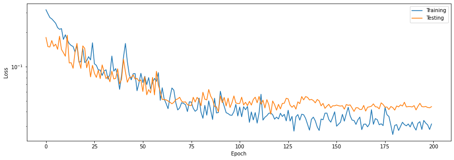
Learning plots.

Plotting the learning curves is as easy as calling stats.plot().

stats.plot(figsize=(15, 5))

Export the best trained model

Load the best model during training and export it as hdf5 network. It is supported by lava.lib.dl.netx to automatically load the network as a lava process.

net.load_state_dict(torch.load(trained_folder + '/network.pt'))
net.export_hdf5(trained_folder + '/network.net')

Operation count of trained model

Here, we compare the synaptic operation and neuron activity of the trained SDNN and an ANN of iso-architecture.

Event statistics on testing dataset

counts = []
for i, (input, ground_truth) in enumerate(test_loader):
    _, count = assistant.test(input, ground_truth)
    count = (count.flatten()/(input.shape[-1]-1)/input.shape[0]).tolist() # count skips first events
    counts.append(count)
    print('\rEvent count : ' + ', '.join([f'{c:.4f}' for c in count]), f'| {stats.testing}', end='')

counts = np.mean(counts, axis=0)

Event count : 2170.5430, 224.2953, 372.4000, 507.9524, 28.2095, 4.7143, 1.0000, 0.1333, 0.4286 | loss =     0.04975 (min =     0.03812)

Event and Synops comparion with ANN

utils.compare_ops(net, counts, mse=stats.testing.min_loss)

|-----------------------------------------------------------------------------|
|                         |          SDNN           |           ANN           |
|-----------------------------------------------------------------------------|
|         |     Shape     |  Events  |    Synops    | Activations|    MACs    |
|-----------------------------------------------------------------------------|
| layer-0 | (100, 33,  3) |  2475.93 |              |       9900 |            |
| layer-1 | ( 49, 16, 24) |   239.46 |    133700.12 |      18816 |     534600 |
| layer-2 | ( 24,  7, 36) |   422.39 |     19395.86 |       6048 |    1524096 |
| layer-3 | ( 22,  4, 64) |   558.71 |    121649.28 |       5632 |    1741824 |
| layer-4 | ( 20,  2, 64) |    29.90 |    321818.47 |       2560 |    3244032 |
| layer-5 | (  1,  1,100) |     4.80 |      2989.97 |        100 |     256000 |
| layer-6 | (  1,  1, 50) |     1.35 |       240.00 |         50 |       5000 |
| layer-7 | (  1,  1, 10) |     0.16 |        13.46 |         10 |        500 |
| layer-8 | (  1,  1,  1) |     0.44 |         0.16 |          1 |         10 |
|-----------------------------------------------------------------------------|
|  Total  |               |  3733.14 |    599807.33 |      43117 |    7306062 |
|-----------------------------------------------------------------------------|


MSE            : 0.038123 sq. radians
Total neurons  : 43117
Events sparsity: 11.55x
Synops sparsity: 12.18x

If you want to learn more about Sigma-Delta neurons, take a look at the Lava tutorial.

Find out more about Lava and have a look at the Lava documentation or dive into the source code.

To receive regular updates on the latest developments and releases of the Lava Software Framework please subscribe to the INRC newsletter.